


TensorFlowクラスタで ディープラーニングの分散処理環境を構築してみる

稲葉 明彦
機械学習とディープラーニング
機械学習という言葉がバズワードになって久しく、今では人工知能という名のもとに、商品のレコメンド機能や自動車の自動運転技術、相場の予測など実社会にも次々に応用され始めている。
その機械学習アルゴリズムの中でも近年特に注目を浴びているのがディープラーニングだ。2016年3月に、Google社が開発したディープラーニングを利用した囲碁用の人工知能「AlphaGo」が世界トップクラスのプロ棋士に勝利したという衝撃的なニュースでも記憶に新しいだろう。
本コラムでは、最新バージョンが先月公開され、AlphaGoでも利用されているGoogleの機械学習フレームワーク「TensorFlow8.0」の目玉機能である分散処理機能についてご紹介する。
TensorFlowとは
ディープラーニングが目覚ましい進化を遂げた2010年代以降、カリフォルニア大学バークレー校の「Caffe」やFacebook社の「Torch」など、さまざまな対応フレームワークが登場している。そんな中、2015年11月に満を持して公開されたGoogle社の「TensorFlow」は、よく整備されたドキュメント類やサンプル、学習状況を手軽に可視化できる「TensorBoard」、そして何より「Google社が自社の数々のプロジェクトで実際に利用している」という信頼性により、今やディープラーニング用フレームワークのデファクトスタンダードになりつつある。
本コラムの趣旨
ディープラーニングは高い学習能力を誇る反面、非常に計算負荷が高くなるアルゴリズムであるため、分散処理が必須である。前述したAlphaGoでもCPU1202個、GPU176個で分散処理を行っている。そこで、本コラムでは実際にバージョン0.8で新たに追加されたクラスタ機能を用いて、TensorFlowの分散処理環境(Distributed TensorFlow)の構築を行い、サンプルを改編したモデルを実行して実際に性能がスケールアウトされることを確認する。構成はパラメーター・サーバー1台、ワーカー・ホスト2台の3台構成となる(下図参照)。
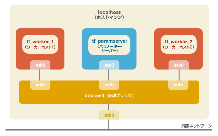
構築はDockerの仮想環境上に行うので一般的なLinuxディストリビューションの環境があれば実施可能である。Windowsでも仮想化支援機能を備えたCPUを搭載したマシンであればHyper-VやVirtualBoxなどのハイパーバイザを用いてLinux環境を用意すれば同様である。もちろんAWSやAzureなどのクラウド上のIaaS環境でも問題ない。ただし、いずれの場合もクラスタの有効性を効果的に確認できるよう各コンテナに1コアずつ指定して割り振るために、クアッドコア以上のCPUであることが望ましい。
注:
- 本来であれば、クラスタ化による性能のスケールアウトの検証を行う場合はその効果を正確に測るため、各マシンは物理的に切り離された形で構築されるべきであるが、本コラムの趣旨はあくまで機能の紹介であるため、利便性を優先し仮想環境で構築を行っている。
- 本コラムはTensorFlowをこれまで使用したことがなく、この機に試してみたいと考えている入門者、またはすでにTensorFlowを利用しておりクラスタ機能の具体的な実装方法を確認したい経験者の方を対象読者として想定しているため、サンプルコードの内容や機械学習およびディープラーニング自体に関する理論的な解説については割愛し、クラスタ機能に関する部分に焦点を絞ってご紹介させていただくこととする。
環境の導入
本節ではTensorFlowクラスタの基盤となるDocker環境の構築、およびTensorFlowイメージの導入を行う。Dockerでの操作は基本的にroot権限が必要となるため、以降のホスト側での作業は全てrootもしくはsudoユーザーで実行されることを想定している点をご注意願いたい。
Dockerのインストールとデーモンの起動
Red Hat系OSの場合(例:CentOS7):
[root@localhost ~]# yum –y epel-release
[root@localhost ~]# yum –y install docker-io
[root@localhost ~]# systemctl start docker
[root@localhost ~]# systemctl status docker	# Dockerデーモンの起動確認
Debian系OSの場合(例:Ubuntu16.04LTS):
root@localhost:~$ apt-get update
root@localhost:~$ apt-get –y install docker.io
root@localhost:~$ service docker start
root@localhost:~$ service docker status	# Dockerデーモンの起動確認
以降では、Red Hat系での環境を想定して話を進めることとする。
TensorFlowイメージのダウンロード
TensorFlowでは公式のDockerイメージが公開されており、面倒な環境構築などをせずに仮想環境上で手軽に利用できるようになっている。下記のコマンドでイメージをダウンロードすることができる。
[root@localhost ~]# docker pull gcr.io/tensorflow/tensorflow:0.8.0
[root@localhost ~]# docker images	# イメージがダウンロードされていることを確認
REPOSITORY 		TAG 	IMAGE ID		CREATED		VIRTUAL SIZE
gcr.io/tensorflow/tensorflow	0.8.0	6365706aad48 	2 weeks ago 		714.1 MB
各コンテナの起動
Dockerコンテナの起動を行う。本コラムで構築する環境では各クラスタのインスタンスはPythonのインタラクティブシェル上で実行するため、各コンテナの起動はそれぞれ別のターミナルを立ち上げて実行していただきたい。
パラメーター・サーバー用コンテナの起動
[root@localhost ~]# docker run -it --name tf_paramserver --rm --cpuset-cpus 0 -h tf_paramserver -v <ホストマシン上の共有ディレクトリのパス>:/tmp gcr.io/tensorflow/tensorflow:0.8.0 /bin/bash
root@tf_paramserver:/notebooks#		# 作成したコンテナに移動した
root@tf_paramserver:/notebooks# ifconfig	# コンテナのIPの確認
eth0      Link encap:Ethernet  HWaddr 02:42:ac:11:00:02
          inet addr:<パラメーター・サーバーのip>  Bcast:0.0.0.0  Mask:255.255.0.0
          inet6 addr: fe80::42:acff:fe11:2/64 Scope:Link
          UP BROADCAST RUNNING MULTICAST  MTU:1500  Metric:1
          RX packets:20 errors:0 dropped:0 overruns:0 frame:0
          TX packets:7 errors:0 dropped:0 overruns:0 carrier:0
          collisions:0 txqueuelen:0
          RX bytes:1584 (1.5 KB)  TX bytes:558 (558.0 B)

lo        Link encap:Local Loopback
          inet addr:127.0.0.1  Mask:255.0.0.0
          inet6 addr: ::1/128 Scope:Host
          UP LOOPBACK RUNNING  MTU:65536  Metric:1
          RX packets:0 errors:0 dropped:0 overruns:0 frame:0
          TX packets:0 errors:0 dropped:0 overruns:0 carrier:0
          collisions:0 txqueuelen:0
          RX bytes:0 (0.0 B)  TX bytes:0 (0.0 B)
ワーカー・ホスト1用のコンテナの起動
[root@localhost ~]# docker run -it --name tf_worker_1 --rm --cpuset-cpus 1 -h tf_worker_1 -v <ホストマシン上の共有ディレクトリのパス>:/tmp gcr.io/tensorflow/tensorflow:0.8.0 /bin/bash
root@tf_worker_1:/notebooks#		# 作成したコンテナに移動した
root@tf_worker_1:/notebooks# ifconfig	# コンテナのIPの確認
eth0      Link encap:Ethernet  HWaddr 02:42:ac:11:00:03
          inet addr: <ワーカー・ホスト1のip>  Bcast:0.0.0.0  Mask:255.255.0.0
          inet6 addr: fe80::42:acff:fe11:3/64 Scope:Link
          UP BROADCAST RUNNING MULTICAST  MTU:1500  Metric:1
          RX packets:13 errors:0 dropped:0 overruns:0 frame:0
          TX packets:7 errors:0 dropped:0 overruns:0 carrier:0
          collisions:0 txqueuelen:0
          RX bytes:1026 (1.0 KB)  TX bytes:558 (558.0 B)

lo        Link encap:Local Loopback
          inet addr:127.0.0.1  Mask:255.0.0.0
          inet6 addr: ::1/128 Scope:Host
          UP LOOPBACK RUNNING  MTU:65536  Metric:1
          RX packets:0 errors:0 dropped:0 overruns:0 frame:0
          TX packets:0 errors:0 dropped:0 overruns:0 carrier:0
          collisions:0 txqueuelen:0
          RX bytes:0 (0.0 B)  TX bytes:0 (0.0 B)
ワーカー・ホスト2用のコンテナの起動
[root@localhost ~]# docker run -it --name tf_worker_2 --rm --cpuset-cpus 2 -h tf_worker_2 -v <ホストマシン上の共有ディレクトリのパス>:/tmp gcr.io/tensorflow/tensorflow:0.8.0 /bin/bash
root@tf_worker_2:/notebooks#		# 作成したコンテナに移動した
root@tf_worker_2:/notebooks# ifconfig	# コンテナのIPの確認
eth0      Link encap:Ethernet  HWaddr 02:42:ac:11:00:04
          inet addr: <ワーカー・ホスト2のip>  Bcast:0.0.0.0  Mask:255.255.0.0
          inet6 addr: fe80::42:acff:fe11:4/64 Scope:Link
          UP BROADCAST RUNNING MULTICAST  MTU:1500  Metric:1
          RX packets:6 errors:0 dropped:0 overruns:0 frame:0
          TX packets:7 errors:0 dropped:0 overruns:0 carrier:0
          collisions:0 txqueuelen:0
          RX bytes:468 (468.0 B)  TX bytes:558 (558.0 B)

lo        Link encap:Local Loopback
          inet addr:127.0.0.1  Mask:255.0.0.0
          inet6 addr: ::1/128 Scope:Host
          UP LOOPBACK RUNNING  MTU:65536  Metric:1
          RX packets:0 errors:0 dropped:0 overruns:0 frame:0
          TX packets:0 errors:0 dropped:0 overruns:0 carrier:0
          collisions:0 txqueuelen:0
          RX bytes:0 (0.0 B)  TX bytes:0 (0.0 B)
docker runコマンドにおける各オプションの概要は下記の通り。
| -it | コンテナ起動後、そのコンテナにアタッチする |
|---|---|
| --name | コンテナ名を指定する |
| --rm | コンテナ終了後、自動的にそのコンテナの削除を行う |
| --cpuset-cpus | 使用するCPUを指定する |
| -h | コンテナのホスト名を指定する |
| -v | ホスト、ゲスト間の共有ディレクトリを指定する |
<ホストマシン上の共有ディレクトリのパス>にはデータや学習結果などを各インスタンスで共有するためのディレクトリを指定する。
各コンテナとも同一のディレクトリを指定すること。読み・書き・実行の権限が付与されていれば場所は特にどこでも問題ない。
また、後の工程で使用するため、ifconfigコマンドの出力より各コンテナのIPを記録しておくこと。
サンプルスクリプトについて
構築したクラスタで実行するモデルには、TensorFlow v0.8にサンプルとして組み込まれているcifar-10のモデルをクラスタ用に修正したものを利用することとする。
cifar-10とは、機械学習モデルの評価によく用いられるデータセットのひとつで、下図のような10カテゴリーに分類された画像が学習用に5万枚、テスト用に1万枚用意されたものである。
cifar-10モデルでは、学習用データで各カテゴリーの特徴を学習させた後、ランダムに選択されたテスト用データのカテゴリーを推測させる問題を解く。 前述したとおり、ディープラーニングの理論的解説についてはここでは述べないが、当該モデルの処理のイメージは下記のようなものになっている。 それではここからクラスタ環境で実行するためのサンプルスクリプトの準備を進める。サンプルスクリプトを実行するクライアントとして新たにターミナルをひとつ立ち上げ、以下のコマンドを実行しパラメーター・サーバー用コンテナにアタッチする。 続いて、基となるcifar10用のモデルをカレントディレクトリーにコピーする。 スタンドアローン用、クラスター用の各パッチファイルをコピー&ペーストにてそれぞれ作成する。 下記のコマンドを実行して、作成したパッチファイルをコピーしたサンプルスクリプトに適用する。 スクリプトの主な変更点はそれぞれ下記の通り。各クラスや関数の定義などについては公式ドキュメントを参照していただきたい。 変更前のモデルではデフォルトで100万ステップの学習を行っているが、これを並列化せずに実行すると最新のCPUを用いても非常に時間がかかってしまう。幸い、今回確認したいのは処理速度だけなので、手軽に実行できるようステップ数を1,000回に設定している。1,000回でも時間がかかる場合はさらに少なくしても問題ない。 パラメーター・サーバーのIPを指定する変数を定義する。 変更前のモデルはマルチGPU対応となっているが、そこで指定される各GPUをクラスタ版ではワーカー・ホストに対応させている。今回は2つのワーカー・ホストを登録するので数量を2に設定。 変更前のモデルではCPUにパラメーター・サーバーの役割に相当する部分を担わせているため、その部分をパラメーター・サーバーに割り当てる。 同様に、変更前のモデルでGPUが担当している箇所をワーカー・ホストに置き換える。 セッションの生成部分。修正前と後で引数の内容が下記のように変更されている。 前節にて作成したスクリプトを実行し、スタンドアローン版、クラスタ版のそれぞれの処理速度を比較する。 スタンドアローン版スクリプトを実行すると、下記のような出力が得られるはずである。 出力の1〜2行目にある通り、初回実行時はcifar-10のデータのダウンロードを行う。2回目以降はダウンロードされたデータを使用するためこの処理が行われることはない。実行速度に関して、筆者の検証環境ではスタンドアローン環境で1秒当たり約95枚の画像を処理することができていた。 続いて、クラスタ版スクリプトを実行するために各インスタンスの起動を行う。前述したとおり、インスタンスごとにそれぞれターミナルを起動して実行すること。 クラスタ版スクリプトの実行結果は下記のようなものとなる。 上記の通り、クラスタ版では1秒当たり約180枚前後の画像を処理できている。スタンドアローン版が約95枚程度だったことを考えるとおよそ2倍の速度となっており、想定通りスケールアウトされていることが確認できる。 本コラムではTensorFlowのクラスタ機能について紹介し、クラスタ用に修正したスクリプトを作成・実行し、性能がスケールすることを確認した。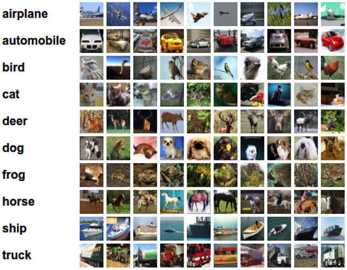
(出典:https://www.tensorflow.org/versions/r0.7/tutorials/deep_cnn/index.html)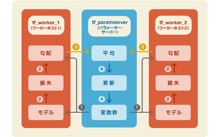
[root@localhost ~]# docker exec –it tf_paramserver /bin/bash
root@tf_paramserver:/notebooks# cp /usr/local/lib/python2.7/dist-packages/tensorflow/models/image/cifar10/cifar10_multi_gpu_train.py .
cifar10_standalone_train.patch
--- cifar10_multi_gpu_train.py  2016-04-13 00:00:00.000000000 +0000
+++ cifar10_standalone_train.py    2016-04-13 00:00:00.000000000 +0000
@@ -54,7 +54,7 @@ FLAGS = tf.app.flags.FLAGS
 tf.app.flags.DEFINE_string('train_dir', '/tmp/cifar10_train',
                            """Directory where to write event logs """
                            """and checkpoint.""")
-tf.app.flags.DEFINE_integer('max_steps', 1000000,
+tf.app.flags.DEFINE_integer('max_steps', 1000,
                             """Number of batches to run.""")
 tf.app.flags.DEFINE_integer('num_gpus', 1,
                             """How many GPUs to use.""")
cifar10_cluster_train.patch
--- cifar10_multi_gpu_train.py  2016-04-13 00:00:00.000000000 +0000
+++ cifar10_cluster_train.py    2016-04-13 00:00:00.000000000 +0000
@@ -49,14 +49,16 @@ from six.moves import xrange  # pylint:
 import tensorflow as tf
 from tensorflow.models.image.cifar10 import cifar10

+PS_NODE = "<パラメーター・サーバーのip>"
+
 FLAGS = tf.app.flags.FLAGS

 tf.app.flags.DEFINE_string('train_dir', '/tmp/cifar10_train',
                            """Directory where to write event logs """
                            """and checkpoint.""")
-tf.app.flags.DEFINE_integer('max_steps', 1000000,
+tf.app.flags.DEFINE_integer('max_steps', 1000,
                             """Number of batches to run.""")
-tf.app.flags.DEFINE_integer('num_gpus', 1,
+tf.app.flags.DEFINE_integer('num_workers', 2,
                             """How many GPUs to use.""")
 tf.app.flags.DEFINE_boolean('log_device_placement', False,
                             """Whether to log device placement.""")
@@ -147,7 +149,7 @@ def average_gradients(tower_grads):

 def train():
   """Train CIFAR-10 for a number of steps."""
-  with tf.Graph().as_default(), tf.device('/cpu:0'):
+  with tf.Graph().as_default(), tf.device('/job:ps/task:0/cpu:0'):
     # Create a variable to count the number of train() calls. This equals the
     # number of batches processed * FLAGS.num_gpus.
     global_step = tf.get_variable(
@@ -171,8 +173,8 @@ def train():

     # Calculate the gradients for each model tower.
     tower_grads = []
-    for i in xrange(FLAGS.num_gpus):
-      with tf.device('/gpu:%d' % i):
+    for i in xrange(FLAGS.num_workers):
+      with tf.device('/job:worker/task:%d/cpu:0' % i):
         with tf.name_scope('%s_%d' % (cifar10.TOWER_NAME, i)) as scope:
           # Calculate the loss for one tower of the CIFAR model. This function
           # constructs the entire CIFAR model but shares the variables across
@@ -231,9 +233,7 @@ def train():
     # Start running operations on the Graph. allow_soft_placement must be set to
     # True to build towers on GPU, as some of the ops do not have GPU
     # implementations.
-    sess = tf.Session(config=tf.ConfigProto(
-        allow_soft_placement=True,
-        log_device_placement=FLAGS.log_device_placement))
+    sess = tf.Session("grpc://%s:2222" % PS_NODE)
     sess.run(init)

     # Start the queue runners.
@@ -249,9 +249,9 @@ def train():
       assert not np.isnan(loss_value), 'Model diverged with loss = NaN'

       if step % 10 == 0:
-        num_examples_per_step = FLAGS.batch_size * FLAGS.num_gpus
+        num_examples_per_step = FLAGS.batch_size * FLAGS.num_workers
         examples_per_sec = num_examples_per_step / duration
-        sec_per_batch = duration / FLAGS.num_gpus
+        sec_per_batch = duration / FLAGS.num_workers

         format_str = ('%s: step %d, loss = %.2f (%.1f examples/sec; %.3f '
                       'sec/batch)')
root@tf_paramserver:/notebooks# cp ./cifar10_multi_gpu_train.py ./cifar10_standalone_train.py
root@tf_paramserver:/notebooks# cp ./cifar10_multi_gpu_train.py ./cifar10_cluster_train.py
root@tf_paramserver:/notebooks# patch ./cifar10_standalone_train.py ./cifar10_standalone_train.patch
patching file cifar10_standalone_train.py
root@tf_paramserver:/notebooks# patch ./cifar10_cluster_train.py ./cifar10_cluster_train.patch
patching file cifar10_cluster_train.py
スタンドアローン版
cifar10_standalone_train.patch:7〜8行目
-tf.app.flags.DEFINE_integer('max_steps', 1000000,
+tf.app.flags.DEFINE_integer('max_steps', 1000,
クラスター版
cifar10_cluster_train.patch:7行目
+PS_NODE = "<パラメーター・サーバーのip>"
cifar10_cluster_train.patch:17〜18行目
-tf.app.flags.DEFINE_integer('num_gpus', 1,
+tf.app.flags.DEFINE_integer('num_workers', 2,
cifar10_cluster_train.patch:26〜27行目
-  with tf.Graph().as_default(), tf.device('/cpu:0'):
+  with tf.Graph().as_default(), tf.device('/job:ps/task:0/cpu:0'):
cifar10_cluster_train.patch:35〜38行目
-    for i in xrange(FLAGS.num_gpus):
-      with tf.device('/gpu:%d' % i):
+    for i in xrange(FLAGS.num_workers):
+      with tf.device('/job:worker/task:%d/cpu:0' % i):
cifar10_cluster_train.patch:46〜49行目
-    sess = tf.Session(config=tf.ConfigProto(
-        allow_soft_placement=True,
-        log_device_placement=FLAGS.log_device_placement))
+    sess = tf.Session("grpc://%s:2222" % PS_NODE)
引数名 説明 修正前 修正後 Target セッションを実行する対象を指定する なし(実行中のプロセス) ホスト:パラメーター・サーバー
ポート:2222
プロトコル:gRPCconfig allow_soft_placemet デバイスの自動割り当てを行うか否か True なし(False) log_device_placement 各演算とテンソルがどのデバイスに割り当てられているかを出力するか否か True なし(False) サンプルプログラムの実行
スタンドアローン版スクリプトの実行
root@tf_paramserver:/notebooks# python cifar10_cluster_train.py
>> Downloading cifar-10-binary.tar.gz 100.0%
Successfully downloaded cifar-10-binary.tar.gz 170052171 bytes.
Filling queue with 20000 CIFAR images before starting to train. This will take a few minutes.
2016-05-08 02:43:30.635849: step 0, loss = 4.68 (12.8 examples/sec; 9.998 sec/batch)
2016-05-08 02:43:45.431379: step 10, loss = 4.66 (98.7 examples/sec; 1.297 sec/batch)
2016-05-08 02:43:58.407859: step 20, loss = 4.64 (98.5 examples/sec; 1.299 sec/batch)
2016-05-08 02:44:11.413918: step 30, loss = 4.62 (98.4 examples/sec; 1.301 sec/batch)
2016-05-08 02:44:24.434746: step 40, loss = 4.60 (98.3 examples/sec; 1.302 sec/batch)
2016-05-08 02:44:37.489811: step 50, loss = 4.59 (98.0 examples/sec; 1.306 sec/batch)
・・・
2016-05-08 03:04:31.150605: step 950, loss = 3.41 (94.4 examples/sec; 1.356 sec/batch)
2016-05-08 03:04:44.737516: step 960, loss = 3.40 (94.4 examples/sec; 1.355 sec/batch)
2016-05-08 03:04:58.297885: step 970, loss = 3.39 (94.4 examples/sec; 1.356 sec/batch)
2016-05-08 03:05:11.861645: step 980, loss = 3.38 (94.5 examples/sec; 1.355 sec/batch)
2016-05-08 03:05:25.418296: step 990, loss = 3.36 (94.4 examples/sec; 1.356 sec/batch)
クラスタ版スクリプトの実行
パラメーター・サーバー用インスタンスの起動
root@tf_paramserver:/notebooks# python	# Pythonのインタラクティブシェルを起動する
>>> import tensorflow as tf	# 以下は起動したPythonのインタラクティブシェル上で実行

cluster = tf.train.ClusterSpec({
	"ps": [
		"<パラメーター・サーバーのip>:2222"
	],
	"worker": [
		"<ワーカー・ホスト1のip>:2222",
		"<ワーカー・ホスト2のip>:2222"
	]})
server = tf.train.Server(cluster, job_name="ps", task_index=0)
ワーカー・ホスト1用インスタンスの起動
root@tf_worker_1:/notebooks# python	# Pythonのインタラクティブシェルを起動する
>>> import tensorflow as tf	# 以下は起動したPythonのインタラクティブシェル上で実行

cluster = tf.train.ClusterSpec({
	"ps": [
		"<パラメーター・サーバーのip>:2222"
	],
	"worker": [
		"<ワーカー・ホスト1のip>:2222",
		"<ワーカー・ホスト2のip>:2222"
	]})
server = tf.train.Server(cluster, job_name="worker", task_index=0)
ワーカー・ホスト2用インスタンスの起動
root@tf_worker_2:/notebooks# python	# Pythonのインタラクティブシェルを起動する
>>> import tensorflow as tf	# 以下は起動したPythonのインタラクティブシェル上で実行

cluster = tf.train.ClusterSpec({
	"ps": [
		"<パラメーター・サーバーのip>:2222"
	],
	"worker": [
		"<ワーカー・ホスト1のip>:2222",
		"<ワーカー・ホスト2のip>:2222"
	]})
server = tf.train.Server(cluster, job_name="worker", task_index=1)
クラスタ版スクリプトの実行
root@tf_paramserver:/notebooks# python cifar10_cluster_train.py
Filling queue with 20000 CIFAR images before starting to train. This will take a few minutes.
Filling queue with 20000 CIFAR images before starting to train. This will take a few minutes.
2016-05-07 20:21:33.712485: step 0, loss = 4.67 (11.7 examples/sec; 10.936 sec/batch)
2016-05-07 20:21:50.442159: step 10, loss = 4.65 (171.5 examples/sec; 0.746 sec/batch)
2016-05-07 20:22:04.883423: step 20, loss = 4.63 (172.6 examples/sec; 0.742 sec/batch)
2016-05-07 20:22:19.511816: step 30, loss = 4.62 (170.4 examples/sec; 0.751 sec/batch)
2016-05-07 20:22:33.988097: step 40, loss = 4.60 (170.8 examples/sec; 0.749 sec/batch)
2016-05-07 20:22:48.366351: step 50, loss = 4.58 (168.9 examples/sec; 0.758 sec/batch)
・・・
2016-05-07 20:44:58.754436: step 950, loss = 3.37 (165.2 examples/sec; 0.775 sec/batch)
2016-05-07 20:45:13.747582: step 960, loss = 3.29 (165.3 examples/sec; 0.774 sec/batch)
2016-05-07 20:45:28.697977: step 970, loss = 3.21 (180.7 examples/sec; 0.708 sec/batch)
2016-05-07 20:45:43.997790: step 980, loss = 3.18 (166.2 examples/sec; 0.770 sec/batch)
2016-05-07 20:45:59.043413: step 990, loss = 3.06 (179.8 examples/sec; 0.712 sec/batch)
また、同じステップ数でも処理できるデータが多くなったので、lossもスタンドアローン版が3.36であったのに対し、クラスタ版では3.06とより低い値になっており、学習が早く進んでいることがわかる。まとめ
今回はDockerを用いた仮想環境上でクラスタを構築したが、Google社では同じく同社で開発しているDockerのオーケストレーションツールであるKubernetesを用いてTensorFlowクラスタの管理しており、実は冒頭のAlphaGoのような大規模なTensor Flowクラスタは今回構築した環境の延長線上にあるともいえる。そういった意味でも、本コラムがこれからますます進化・発展していくだろうTensorFlowに対する皆さまの理解の一助になれたなら幸いである
Tweet